wav_files =[x.replace('.txt', '.wav') forx intxt_files]

　　# Load audio and text into memory

　　(audio, text) =get_audio_and_tran(

　　txt_files,

　　wav_files,

　　_numcep,

　　_numcontext)

特征表示

为了让机器识别音频数据，数据必须先从时域转换为频域。有几种用于创建音频数据机器学习特征的方法，包括任意频率的 binning（如 100Hz），或人耳能够感知的频率的 binning。这种典型的语音数据转换需要计算 13 位或 26 位不同倒谱特征的梅尔倒频谱系数（MFCC）。在转换之后，数据被存储为时间（列）和频率系数（行）的矩阵。

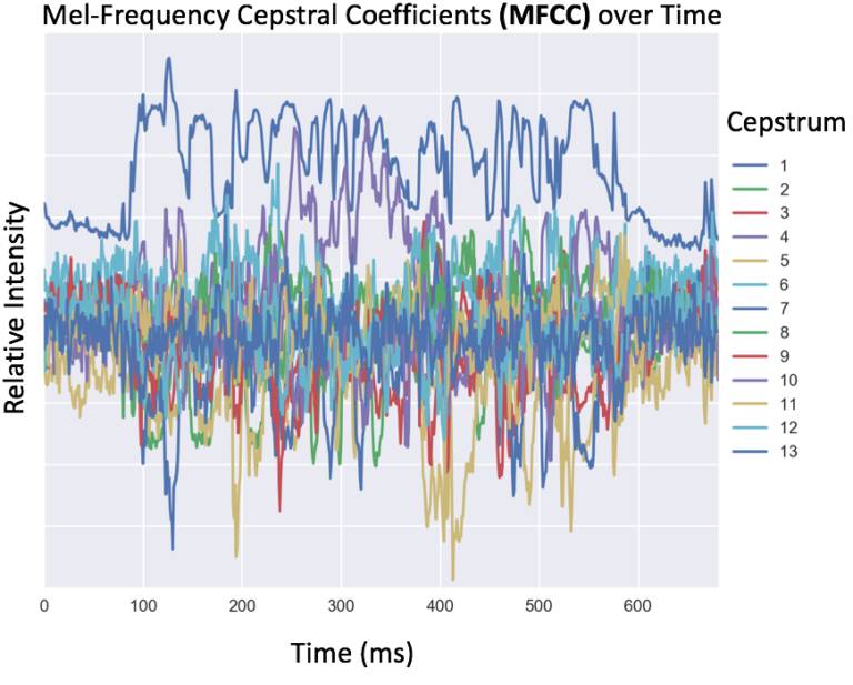
因为自然语言的语音不是独立的，它们与字母也不是一一对应的关系，我们可以通过训练神经网络在声音数据上的重叠窗口（前后 10 毫秒）来捕捉协同发音的效果（一个音节的发音影响了另一个）。以下代码展示了如何获取 MFCC 特征，以及如何创建一个音频数据的窗口。

　　# Load wav files

　　fs, audio =wav.read(audio_filename)

　　# Get mfcc coefficients

　　orig_inputs =mfcc(audio, samplerate=fs, numcep=numcep)

　　# For each time slice of the training set, we need to copy the context this makes

　　train_inputs =np.array([], np.float32)

　　train_inputs.resize((orig_inputs.shape[0], numcep +2*numcep *numcontext))

　　fortime_slice inrange(train_inputs.shape[0]):

　　# Pick up to numcontext time slices in the past,

　　# And complete with empty mfcc features

　　need_empty_past =max(0, ((time_slices[0] +numcontext) -time_slice))

　　empty_source_past =list(empty_mfcc forempty_slots inrange(need_empty_past))

　　data_source_past =orig_inputs[max(0, time_slice -numcontext):time_slice]

　　assert(len(empty_source_past) +len(data_source_past) ==numcontext)

　　...

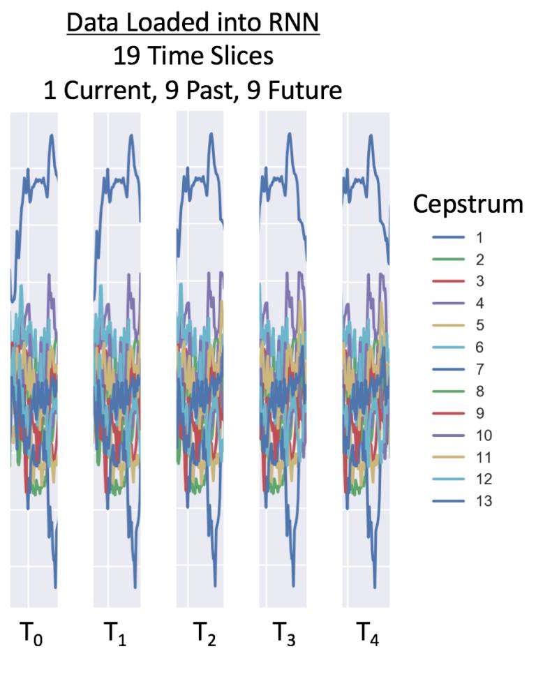
对于这个 RNN 例子来说，我们在每个窗口使用前后各 9 个时间点——共 19 个时间点。有 26 个倒谱系数，在 25 毫秒的时间里共 494 个数据点。根据数据采样率，我们建议在 16,000 Hz 上有 26 个倒谱特征，在 8,000 Hz 上有 13 个倒谱特征。以下是一个 8,000 Hz 数据的加载窗口：

如果你希望了解更多有关转换数字音频用于 RNN 语音识别的方法，可以看看 Adam Geitgey 的介绍：

对语音的序列本质建模

长短期记忆（LSTM）是循环神经网络（RNN）的一种，它适用于对依赖长期顺序的数据进行建模。它对于时间序列数据的建模非常重要，因为这种方法可以在当前时间点保持过去信息的记忆，从而改善输出结果，所以，这种特性对于语音识别非常有用。如果你想了解在 TensorFlow 中如何实例化 LSTM 单元，以下是受 DeepSpeech 启发的双向循环神经网络（BiRNN）的 LSTM 层示例代码：

　　with tf.name_scope('lstm'):

　　# Forward direction cell:

　　lstm_fw_cell =tf.contrib.rnn.BasicLSTMCell(n_cell_dim, forget_bias=1.0, state_is_tuple=True)

　　# Backward direction cell:

　　lstm_bw_cell =tf.contrib.rnn.BasicLSTMCell(n_cell_dim, forget_bias=1.0, state_is_tuple=True)

　　# Now we feed `layer_3` into the LSTM BRNN cell and obtain the LSTM BRNN output.

　　outputs, output_states =tf.nn.bidirectional_dynamic_rnn(

　　cell_fw=lstm_fw_cell,

　　cell_bw=lstm_bw_cell,

　　# Input is the previous Fully Connected Layer before the LSTM

　　inputs=layer_3,

　　dtype=tf.float32,

　　time_major=True,

　　sequence_length=seq_length)

　　tf.summary.histogram("activations", outputs)

关于 LSTM 网络的更多细节，可以参阅 RNN 与 LSTM 单元运行细节的概述：

此外，还有一些工作探究了 RNN 以外的其他语音识别方式，如比 RNN 计算效率更高的卷积层：https://arxiv.org/abs/1701.02720

训练和监测网络

转载请注明出处。